Modelling Solutions for Natural Water Bodies

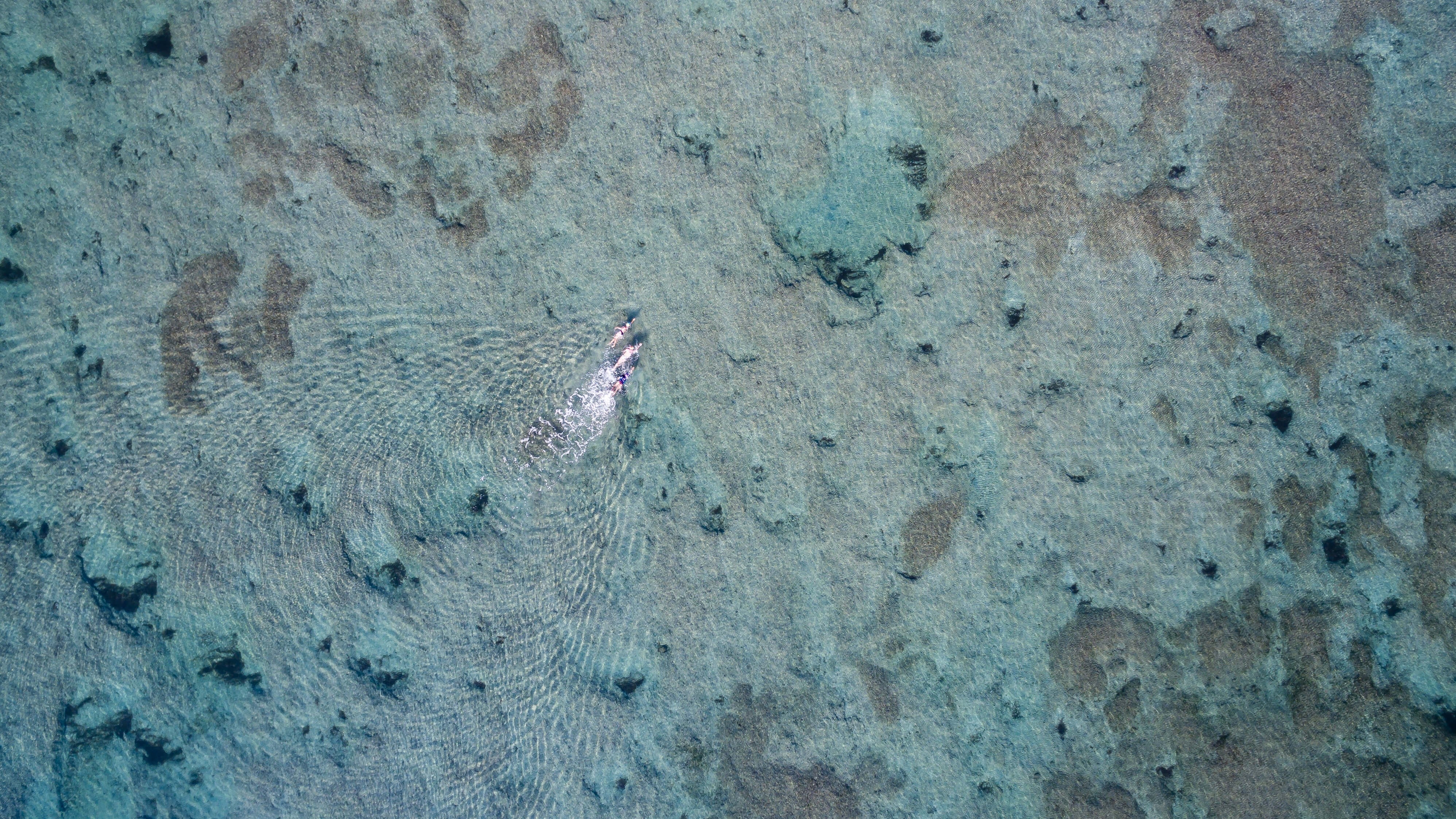
We begin with the following brief: jump yourself into a paraglider and take flight over the ocean. What do you see? [Figs. 1 & 2] The sea, firstly. Hopefully. But what is that murky patch? Sea weed? How deep down is it should you wish to go for a swim? Is that a chest of gold treasure glinting back at you in the sunlight?

To answer these questions, without getting your hands dirty, one could write a computer model to simulate what is seen in a water body from above, the idea being then to ‘forecast’ what would be seen given the local conditions such as cloud cover, time of day, water turbidity, or depth of the water bed. For example, one could input the optical properties attached to a clump of sea weed of that shape and thus predict its depth. Or perhaps the model would point out that it is most likely an oil spill being observed when reconciling its reflective properties.

Such a computer model is based on the transfer of light in water and developing such is one of the research focuses of the TEAM-A project. In this article, we describe the basic principles of radiative transfer within a water body and establish a ‘fast’ mathematical procedure to solve its equation of motion. This solution shall be in the spotlight of our present discussion; it is known as the invariant imbedding method and was first derived analytically by Preisendorfer [5]. This method supersedes its peers, such as Monte Carlo simulation, vastly in computational efficiency. In its present form, the invariant imbedding method and algorithmic application has been developed by Mobley [2] and Mobley et. al. [3]. A full technical account is given in [4]. Our aim is to build on these works to handle new and exotic scenarios.

The quantity which we want to obtain from such a model is the radiance; this is by definition the amount of power transferred per unit area, at a given point in the water body, with respect to infinitesimal increments in bandwidth and, characteristically, the angle of entrance. The governing equation of motion for the system, the so-called radiative transfer equation (RTE), is derived by equating the substantive derivative of the radiance to the various terms which physically account for its rate of change: scattering, absorption, internal sources etc. The fundamental principle of radiative transfer – a physical assumption which we then impose – is that its propagation is linear; response radiances at a given point are linear functions of the incident radiances.

To solve the RTE, let us impose a handful of assumptions on the system (of light travelling in water) itself.  Suppose that that the water body is horizontally homogenous: that radiative transfer is unchanging over time. Then the RTE simplifies to an expression equating the total rate of change with respect to vertical depth of the radiance. With boundary conditions imposed at the surface and the bottom, this constitutes a two-point boundary value problem, at least when averaged over the hemisphere of observation. Compared with initial value problems (IVPs), for which a single boundary condition is imposed on a system of differential equations, deriving an analytic solution for a two-point boundary value problem is difficult. Traditionally, a solution would be obtained by solving the RTE itself within the water body given, using, for example, Monte Carlo methods.  It is the invariant imbedding method which shall partition the RTE into more manageable IVPs.

Let us now explain the concept of invariant imbedding. For starters, what remains invariant and what is imbedded? This is best illustrated by analogy with the work of Ambarzumian [1], whose ideas formed the basis of this technique. Ambarzumian considered an infinitely deep stellar atmosphere and sought to compute its reflectance. His postulation was that this reflectance would remain invariant in the atmosphere when an additional infinitesimal layer was added (just as the number of guests did not change when Hilbert checked in new arrivals to his infinite Grand Hotel [6]). The problem of computing the reflectance at a point is then imbedded into the problem of computing the reflectance at an infinitesimally close point. He established a functional equation for the reflectance at these points. Assuming that the point is infinitely deep within the atmosphere, Ambarzumian could then solve for the reflectance directly without ever having to solve the RTE at all.

Where does Mobley’s [4] much more elaborate construction differ? The sea is not infinitely deep and hence any small change in depth is sizeable against the overall depth. A consequence of this is that the functional equations we derive for reflectance, transmittance, and internal source terms depend also on their total derivatives with respect to depth in the water body. These constitute a system of IVPs which are computationally speedy to solve – these are also the features of the system which remain invariant upon adding infinitesimal lays of water to the system. Once again, these are solved for without ever having to solve the RTE itself. We finally obtain the radiance via the fundamental principal of radiative transfer theory: this links the response radiance linearly with the reflectance etc. in terms of the incident radiances.

Future prospects for the evolution of this theory are exciting from both engineering and environmental perspectives. Allowing the model to learn with data sets and real life images would help produce a powerful predictive tool to answer a multitude of nautical questions. On the other hand, the mathematical techniques developed in the literature lend themselves to applications in different systems where the fundamental assumptions may be applied analogously.

References

[1] Ambarzumian, V.A., 1943. Diffuse reflection of light by a foggy medium, Compt. rend. (Doklady), Acad. Sci., U.S.S.R., 38, 229.

[2] Mobley, C.D., 1989. A numerical model for the computation of radiance distributions in natural waters with wind-roughened surfaces, Limnol. Oceanogr., 34(8), 1473-1483.

[3] Mobley, C.D., B. Gentili, H.R. Gordon, Z. Jin, G.W. Kattawar, A. Morel, P. Reinersman, K. Stammes, and R.H. Stavn, 1993. Comparison of numerical models for computing underwater light fields, Appl. Opt., 32(36), 7484-7505.

[4] Mobley, C.D., Light and Water, Academic Press, 1994.

[5] Preisendorfer, R.W., 1958. Unified irradiance equations, Scripps Inst. Oceanogr. Ref. 58-43, Univ. of Calif., San Diego.

[6] Wikipedia, https://en.wikipedia.org/wiki/Hilbert%27s_paradox_of_the_Grand_Hotel