Image Analysis

The Bioimaging Centre is equipped with 2 high-end workstation PCs within the research facility. The workstations have the latest versions of image-processing software (see table below), which enable state-of-the-art image analysis and processing of image data.

Please contact our Bioimaging staff if you are interested in using our workstations.

The Imaris F1 package contains the following modules:

Fluorescence recovery after photobleaching - FRAP

FRAP (Fluorescence recovery after photobleaching) is a method that allows one to determine the movement of cellular molecules. Frap is a multistep process (Figure 1), which involves 1. Capturing images with a low light to establish the initial fluorescence of the sample. 2. Then a high level of light exposure is carried out, to a region of interest (ROI), which is done to bleach the sample. 3. Finally, the last step involves using a low level of light, which is enough to excite, but not so high to cause further bleaching. This gains insight into the movement of any molecules repopulating the ROI over time. Other variations of FRAP are also possible with our systems, such as Fluorescence loss in photobleaching (FLIP), Inverse FRAP (iFRAP) and Fluorescence Localization After Photobleaching (FLAP).

Applications:

• Membrane mobility studies
• Studies of protein binding
• Studies of non-membrane protein behavior

If you want to apply this method please feel free to discuss the options the Bioimaging Centre can offer you.

FRAP can be utilised with the following microscope systems of our research facility:

• Zeiss LSM 880 with Airyscan
• Leica TCS SP8
• Spinning disc (Olympus IX81)
• Olympus IX81 widefiled system

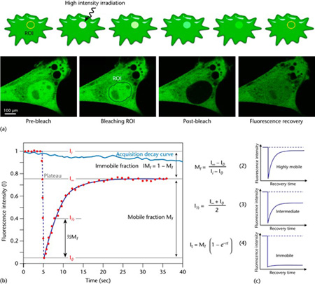
Figure 1 Schematic representation of a FRAP experiment. (a) A region of interest (ROI) is selected, bleached with an intense laser beam, and the fluorescence recovery in the ROI is measured over time. Below: actual experiment in a myoblast cell line (myo3) homogenously expressing GFP-Myosin III before bleaching. (b) From the initial (pre-bleach) fluorescence intensity (Ii), the signal drops to a low value (I0) as the high-intensity laser beam bleaches fluorochromes in the ROI. Over time, the signal recovers from the post-bleach intensity (I0) to a maximal plateau value (IN). From this plot and eqn (2) and eqn (3), the mobile fraction (Mf), immobile fraction (IMf), and I1 can be calculated. Light blue line: reference photobleaching curve to correct for fluorescence loss during data acquisition. The information from the recovery curve (from I0 to IN) can be used to determine the diffusion constant and the binding dynamics of fluorescently labelled proteins. A more absolute way of obtaining the half-life and immobile/mobile fractions, which is also suitable for automation, is through nonlinear curve fitting of the experimental data points using the simple exponential eqn (4). (c) The curve directly shows the extent of the mobility observed. This figure and text is from Ishikawa-Ankerhold, Ankerhold & Drummen, (2014), which was originally modified from Ishikawa-Ankerhold, Ankerhold & Drummen, (2012).

Useful links

Measuring Dynamics: Photobleaching and Photoactivation (Jennifer Lippincott-Schwartz (National Institute of Health - NIH); https://www.youtube.com/watch?v=t91gwtdE7L0

Introduction to Fluorescence Recovery after Photobleaching (FRAP); https://www.embl.de/eamnet/downloads/courses/FRAP2005/tzimmermann_frap.pdf

References

Ishikawa-Ankerhold, H.C., Ankerhold, R. & Drummen, G.P.C. (2012) Advanced fluorescence microscopy techniques-FRAP, FLIP, FLAP, FRET and FLIM. Molecules. 17 (4), pp. 4047–4132.

McNally, J.G. (2008) Quantitative FRAP in Analysis of Molecular Binding Dynamics In Vivo. Methods in Cell Biology. 85pp. 329–351.

Stavreva, D.A. & McNally, J.G. (2003) Fluorescence Recovery after Photobleaching (FRAP) Methods for Visualizing Protein Dynamics in Living Mammalian Cell Nuclei. Methods in Enzymology. 375pp. 443–455.

Sprague, B.L. & McNally, J.G. (2005) FRAP analysis of binding: Proper and fitting. Trends in Cell Biology. 15 (2), pp. 84–91.

Fluorescence Correlation Spectroscopy (FCS) and subsidiary methods

Fluorescence correlation spectroscopy (FCS) is a method that offers insight into the diffusion and localised concentration behaviour, of particles of interest (molecules, proteins). FCS is achieved via a correlative analysis of temporal fluctuation of fluorescence intensity, within an observation volume (Figure 1). The methods tracks temporal changes in light intensity, caused by single fluorophores migrating through the observation window. These intensity fluctuations can then be quantified by temporally auto-correlating the recorded intensity signal, which derives the number of particles and the diffusion time within the observation window. From this parameter biochemical parameters, such as the concentration and size and shape and the viscosity of the local environment can be derived.

Applications:

• Average absolute concentrations
• Diffusion coefficients
• Hydrodynamic radii
• Kinetic chemical reaction rates
• Singlet-triplet dynamics
• Binding ratios (FCCS)

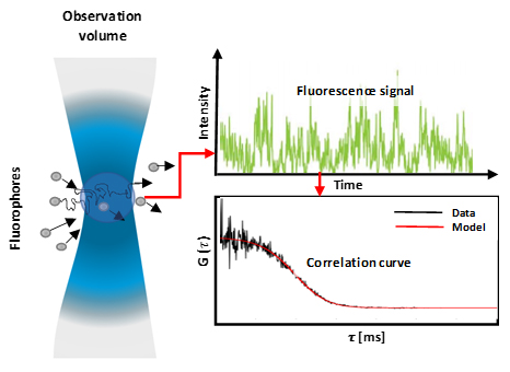
Figure 1: Fluorescent molecules diffusing into and out of an observation volume (diffraction-limited) which results in a fluctuating fluorescence signal which corresponds to the fluctuating particle number. These fluctuations are then analysed by calculating auto-correlation curves. The molecules' diffusion coefficient is inversely proportional to the width of the correlation curve, and the concentration is inversely proportional to the amplitude of the curve.

FCCS

Fluorescence (Cross-) Correlation Spectroscopy (FCCS) is an offspring method of FCS, which correlates light emission derived from two different fluorophores, which is recorded in two separate channels. Through this, it is possible to determine the degree of interaction between two molecules of interest.  As such, FCCS lends itself to gaining information about low molecular concentration within living systems.

Useful links

Optimized processing and analysis of conventional confocal microscopy generated scanning FCS data:

https://www.youtube.com/watch?v=o8frXKd-ynI&t=135s

Fluorescence Correlation Spectroscopy:

https://www.leica-microsystems.com/science-lab/fluorescence-correlation-spectroscopy/

-

References

Buschmann, V., Krämer, B., Koberling, F., Macdonald, R. & Rüttinge, S. (2007) Quantitative FCS: Determination of the Confocal Volume by FCS and Bead Scanning with the MicroTime 200. AppNote Quantitative FCS. pp. 1–8.

Schwille, P. & Haustein, E. (2001) Fluorescence correlation spectroscopy. An introduction to its concepts and applications. Doi:10.1002/Lpor.200910041. pp. 1–33.

Ishikawa-Ankerhold, H.C., Ankerhold, R. & Drummen, G.P.C. (2012) Advanced fluorescence microscopy techniques-FRAP, FLIP, FLAP, FRET and FLIM. Molecules. 17 (4), pp. 4047–4132.

Fluorescent Lifetime Imaging (FLIM) and subsidiary methods

Fluorescence Lifetime Imaging (FLIM) is a method that builds a contrast image based on the differences in the fluorescence decay rate, as fluorophores return to their ground state post excitation. As such, an image is created from the fluorophores lifetime, rather than its intensity. Specifically, this has the advantage of minimizing artifacts that are often introduced from light scattering and quenching.

Applications:

• Tissue characterization by autofluorescence
• Discrimination of multiple labels or background removal
• Detection of conformational changes
• Detection of molecular interactions
• Local environment sensing
• Lifetime or intensity FRET (FLIM-FRET)
• Binding studies
• Protein folding
• Studies of molecular motors

If you want to learn more about this method please contact a member of Bioimaging to discuss possible options within our research facility.

FLIM can be applied with the following microscope systems:

• Leica SPX HyVolution II

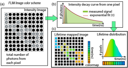
 Figure: Fluorescence lifetime Imaging. In a FLIM image, every pixel records the intensity decay curve at picosecond resolution. The image mapping the total number of photons from the entire recorded time is called the intensity image (A). Each pixel has an intensity decay curve that can be fit to an exponential function after a deconvolution step with the instrument’s timing response function (B). The fitting result from each pixel, the mean lifetime value can be color mapped into an image and the histogram can be plotted in parallel as shown in panel (C). This figure and text is from Chacko & Eliceiri, (2019).

Useful links

Microscopy: Fluorescence Lifetime Imaging Microscopy (FLIM) (Philippe Bastiaens):

https://www.youtube.com/watch?v=haE-ejlYPxw&t=1069s

FLIM and FCS introduction:

https://www.youtube.com/watch?v=bo2oTCUaFb8&t=26s

Introduction to fluorescence lifetime imaging:

https://www.youtube.com/watch?v=k8ar_M-MVao

References

Chacko, J. V. & Eliceiri, K.W. (2019) Autofluorescence lifetime imaging of cellular metabolism: Sensitivity toward cell density, pH, intracellular, and intercellular heterogeneity. Cytometry Part A. 95 (1), pp. 56–69.

Brismar, H. & Ulfhake, B. (1997) Fluorescence lifetime measurements in confocal microscopy of neurons labeled with multiple fluorophores. Nature Biotechnology. 15 (4), pp. 373–377.

Trautmann, S. (2013) Fluorescence Lifetime Imaging (FLIM) in Confocal Microscopy Applications: An Overview.